Thursday, January 31, 2008
Falls of wicket
This is a follow-up to my post on the "fow-average" of openers. Soulberry wanted to see what the average fall of wicket was for non-openers. To make things easier for me, I've split it up by position.
Note that I found a bug in my earlier code, so the list of the top openers has shuffled around a little, though Russel Arnold remains on top. In the tables below I give the number of innings (less any not-outs which didn't see a wicket fall) and the fow-average. Note that for the non-openers, I've subtracted off the wicket that the batsman came in at. Qualification: 15 innings. (Edit: Richie Richardson's figures below are wrong, and Michael Clarke's might be as well. My lazy code got them mixed up with Viv Richards and Stuart Clark.)
There's a rather conspicuous absentee amongst the number threes. I went through Bradman's innings, and when he made a big score he was often part of a large partnership, so that he actually didn't see too many wickets fall. His fow-average at number three is 2,45.
Samir also wanted to see average team runs scored while the batsman is at the crease. I did mean to calculate this, but I forgot until after I'd made my spreadsheets. I think the above tables are interesting enough as it is though. There are several players that you would expect to have "held the innings together" often.
Note that I found a bug in my earlier code, so the list of the top openers has shuffled around a little, though Russel Arnold remains on top. In the tables below I give the number of innings (less any not-outs which didn't see a wicket fall) and the fow-average. Note that for the non-openers, I've subtracted off the wicket that the batsman came in at. Qualification: 15 innings. (Edit: Richie Richardson's figures below are wrong, and Michael Clarke's might be as well. My lazy code got them mixed up with Viv Richards and Stuart Clark.)
opener                            number 3
Russel Arnold           15  3,22  George Headley          32  3,71
Raman Subba Row         16  2,97  George Gunn             16  2,94
Ravi Shastri            26  2,95  Allan Border            37  2,92
Bill Woodfull           43  2,90  Wally Hammond           50  2,91
Glenn  Turner           66  2,87  Richie Richardson       174 2,89
Bruce Mitchell          48  2,78  Alvin Kallicharran      25  2,84
Arthur Shrewsbury       18  2,78  Rahul Dravid            143 2,84
Jackie McGlew           58  2,74  Ken Barrington          40  2,78
Dennis Amiss            69  2,66  Eric Rowan              20  2,71
Chris Tavaré            33  2,63  Lindsay Hassett         19  2,68

number 4                          number 5
Dean Jones              18  3,20  Michael Clarke          31  3,12
Rahul Dravid            18  3,11  Jimmy Adams             29  3,04
Rajin Saleh             23  2,91  Shivnarine Chanderpaul  80  2,97
Jacques Kallis          96  2,84  Kevin Pietersen         25  2,84
Geoff Howarth           17  2,76  Dilip Vengsarkar        30  2,77
Vijay Hazare            35  2,69  Yashpal Sharma          29  2,70
Brian Hastings          29  2,58  Steve Waugh             138 2,69
Monty Noble             23  2,57  Andy Flower             80  2,69
Herbie Taylor           23  2,57  Ken Viljoen             16  2,69
Richie Richardson       19  2,53  John Crawley            15  2,62

number 6
Joe Solomon             16  3,41
Trevor Bailey           38  3,37
Imran Khan              22  3,23
Nawab of Pataudi        21  2,86
Hashan Tillakaratne     72  2,86
Jimmy Adams             31  2,81
Shivnarine Chanderpaul  39  2,75
Allan Border            58  2,74
Les Ames                17  2,68
Dattu Phadkar           20  2,68
There's a rather conspicuous absentee amongst the number threes. I went through Bradman's innings, and when he made a big score he was often part of a large partnership, so that he actually didn't see too many wickets fall. His fow-average at number three is 2,45.
Samir also wanted to see average team runs scored while the batsman is at the crease. I did mean to calculate this, but I forgot until after I'd made my spreadsheets. I think the above tables are interesting enough as it is though. There are several players that you would expect to have "held the innings together" often.
Tuesday, January 29, 2008
1800's first-class cricket in England: bowlers
This is Part 4 in my series on 1800's cricket in England.
1 - data
2 - classification of matches
3 - filling in the gaps
4 - bowlers
5 - batsmen
6 - bowlers across eras
7 - batsmen across eras
8 - all-rounders (across eras)
9 - wicket-keepers
(Edit: My code at first counted "absent" as a nought not out. This has been fixed. All it does is decrease of new innings and not-out tallies.)
In this post I apply the method detailed in Part 3 to all first-class scorecards with missing data. But first I have to make a small confession — the method I've used is surely not the best one. The scorecards with missing data come in (mostly) two types. The earliest scorecards only credit bowlers with bowled dismissals, and do not record the runs conceded by bowlers (this is a typical example). Later scorecards give full credit to bowlers for their dismissals, but don't record the runs conceded (this is a typical example). There are also five matches where the runs conceded are recorded but bowlers aren't given credit for catches, etc.
The method in Part 3 dealt only with the first type of scorecard. With the second type of scorecard, you should be able to get better estimates of the bowling averages, since you have more data (namely, how many wickets each bowler took). But when I tried to apply a similar method to these scorecards (finding the average percentage of team runs conceded by bowlers who took 1 wicket, bowlers who took 2 wickets, etc.), I got results that were biased in favour of regular wicket-takers. The top 18 wicket-takers in the test dataset had estimates of bowling averages that were too low, with the errors ranging from 0,2% to almost 23%. The (justified) fudge factor used in the previous method makes the estimates even lower!
I don't know (yet?) how to fix this. There must surely be a better, more sophisticated model to estimate runs conceded — you shouldn't get worse results with more data! But since that's what's happening for me, I've instead ignored all the non-bowled dismissals for these scorecards, and applied the method used on the early scorecards. I've then scaled up the estimated runs conceded and estimated wickets so that the wicket tally matches reality.
So, onto the results! In the various tables that follow, I give the start and end years of the career, matches (these may not agree with the usual sources, since I exclude matches that weren't eleven-a-side), wickets, runs conceded, bowling average, +/- %; and then batting stats (for which we have complete data): innings, not-outs, runs, average.
Note 1: If there is a decimal comma in the wickets tally, then it is almost certainly an underestimate. How big an underestimate I don't know. In my test dataset, one bowler's estimated wicket tally was 47% below what it should have been. Despite this, the estimate of the average was only out by just over 7%. For other bowlers, the wickets estimate was within 2% of reality. The lesson here is not to rely on my wicket estimates.
Note 2: One of the columns is called +/- %. About 80% of the estimated averages should fall inside the estimated averages, plus or minus the given percent. If the bowler only ever had bowleds credited to him, this value is 10%.
The first table gives the leading bowlers of the 1800's in England by bowling average. Qualification (for this table and all that follow): 200 wickets.
Note that this doesn't mean that James Cobbett had the lowest average of the 1800's — if the estimate was particularly bad, it might be up around 10. This would still be one of the lowest ever, of course. Cobbett was a round-arm spin bowler.
Second on the table is William Lillywhite, a medium-pace round-arm bowler. His wicket tally is enormous.
Third is Samuel Redgate, a fast bowler who we can thank for batting pads, along with Alfred Mynn (tenth on the table). These two were the fastest bowlers of their day, but Mynn was also a pretty good batsman. They squared off against each other in the North v South game of 1836. Mynn had hurt his ankle before play started, but nevertheless batted at 5 in South's second innings. Redgate repeatedly hit Mynn on his unprotected legs, damaging them to the point where amputation was considered. In what must be one of the most courageous innings of all-time, Mynn struck an unbeaten century (the only century of his first-class career), before being sent to London for medical treatment. After this, batsmen started wearing leg guards. You can read about this innings in more detail here.
James Broadbridge comes in fifth. This average-estimating exercise is particularly useful for the Sussex round-armer — in the standard sources his average is given as 18,62. This very wrong figure is based on just 14 of his career wickets, which total over 400!
The ninth player in the table above is Thomas Nixon, a round-arm slow bowler whose first-class career comprised mostly matches for the MCC. You'll note that the +/- % figure is given as 5,0; this means that roughly half of his runs conceded came in matches where this was recorded. This gives us a useful check: we know that his average in these matches was 10,12. Since the estimated average is 10,0, it looks like the estimate is pretty good.
For what it's worth, the next table shows the leading bowlers by wickets taken. Since the amount of first-class cricket increased over the course of the 19th century, the top of the list is dominated by people who played close to 1900.
WG rather stands out in this list. Not only did he take more than 500 more first-class wickets than anyone else in England in the 1800's, but he did it while averaging over 40 with the bat.
Lillywhite's wickets estimate is almost certainly low, and he should be at least one rank higher. He might deserve to he higher still, but we can't know for sure.
To have a look at some more early bowlers, here's a table with players ordered by the starting year of their careers.
William Lambert was, along with Beauclerk, one of the stand-out all-rounders of the early 19th century. These two have similar averages, both for batting and bowling. The bowling average of around 12,5 is about typical for the era, which was very low-scoring. That should put a batting average of over 27 into some perspective. Lambert was, however, banned for life for match-fixing.
Lord Frederick Beauclerk is perhaps my favourite character in cricket history. Not only was he a Lord, a title sadly absent from modern English cricketers, but he was the golden boy of the first part of the 19th century (see his picture here). Not only was he an outstanding all-rounder, but he embodied the spirit of cricket so lacking in today's players. A clergyman, he claimed to make £600 a year from betting on cricket. He was unassuming when batting — (according to his Wikipedia article at least) he used to place an expensive watch on the middle stump. He was a "foul-mouthed, dishonest man who was one of the most hated figures in society ... he bought and sold matches as though they were lots at an auction".
You may have noticed that, along with the leading wicket-takers being from near 1900, the leading averages are mostly from around the second quarter of the century. Adjusting the bowling averages for era will be the subject of Part 6. A suivre !
If your favourite 19th century bowler with missing data has been omitted from the tables above, you can find him in the table below, which lists all bowlers whose averages needed some estimating. They are ordered by the starting year of their first-class careers.
1 - data
2 - classification of matches
3 - filling in the gaps
4 - bowlers
5 - batsmen
6 - bowlers across eras
7 - batsmen across eras
8 - all-rounders (across eras)
9 - wicket-keepers
(Edit: My code at first counted "absent" as a nought not out. This has been fixed. All it does is decrease of new innings and not-out tallies.)
In this post I apply the method detailed in Part 3 to all first-class scorecards with missing data. But first I have to make a small confession — the method I've used is surely not the best one. The scorecards with missing data come in (mostly) two types. The earliest scorecards only credit bowlers with bowled dismissals, and do not record the runs conceded by bowlers (this is a typical example). Later scorecards give full credit to bowlers for their dismissals, but don't record the runs conceded (this is a typical example). There are also five matches where the runs conceded are recorded but bowlers aren't given credit for catches, etc.
The method in Part 3 dealt only with the first type of scorecard. With the second type of scorecard, you should be able to get better estimates of the bowling averages, since you have more data (namely, how many wickets each bowler took). But when I tried to apply a similar method to these scorecards (finding the average percentage of team runs conceded by bowlers who took 1 wicket, bowlers who took 2 wickets, etc.), I got results that were biased in favour of regular wicket-takers. The top 18 wicket-takers in the test dataset had estimates of bowling averages that were too low, with the errors ranging from 0,2% to almost 23%. The (justified) fudge factor used in the previous method makes the estimates even lower!
I don't know (yet?) how to fix this. There must surely be a better, more sophisticated model to estimate runs conceded — you shouldn't get worse results with more data! But since that's what's happening for me, I've instead ignored all the non-bowled dismissals for these scorecards, and applied the method used on the early scorecards. I've then scaled up the estimated runs conceded and estimated wickets so that the wicket tally matches reality.
So, onto the results! In the various tables that follow, I give the start and end years of the career, matches (these may not agree with the usual sources, since I exclude matches that weren't eleven-a-side), wickets, runs conceded, bowling average, +/- %; and then batting stats (for which we have complete data): innings, not-outs, runs, average.
Note 1: If there is a decimal comma in the wickets tally, then it is almost certainly an underestimate. How big an underestimate I don't know. In my test dataset, one bowler's estimated wicket tally was 47% below what it should have been. Despite this, the estimate of the average was only out by just over 7%. For other bowlers, the wickets estimate was within 2% of reality. The lesson here is not to rely on my wicket estimates.
Note 2: One of the columns is called +/- %. About 80% of the estimated averages should fall inside the estimated averages, plus or minus the given percent. If the bowler only ever had bowleds credited to him, this value is 10%.
The first table gives the leading bowlers of the 1800's in England by bowling average. Qualification (for this table and all that follow): 200 wickets.
name          start end   mat wkts    runs    avg   +/- %   inns  no  runs  avg
J Cobbett     1826  1841  94  556,3   4598,7  8,3   9,7     162   16  1437  9,84
FW Lillywhite 1825  1851  220 1599,8  14181,1 8,9   8,5     390   84  2203  7,20
S Redgate     1830  1846  74  414,0   3775,2  9,1   8,0     133   23  957   8,70
J Broadbridge 1814  1840  90  405,6   3699,7  9,1   9,9     163   21  2368  16,68
J Bayley      1822  1850  81  358,7   3500,5  9,8   9,3     140   17  905   7,36
G Freeman     1865  1880  44  288     2849,2  9,9   0,2     70    3   918   13,70
WR Hillyer    1835  1853  216 1407,3  14061,5 10,0  7,1     386   62  2544  7,85
J Wisden      1845  1863  175 1036,5  10356,9 10,0  3,4     305   29  4020  14,57
T Nixon       1841  1859  50  250     2503,5  10,0  5,0     83    17  300   4,55
A Mynn        1832  1859  200 1059,9  10940,1 10,3  7,0     372   24  4749  13,65
Note that this doesn't mean that James Cobbett had the lowest average of the 1800's — if the estimate was particularly bad, it might be up around 10. This would still be one of the lowest ever, of course. Cobbett was a round-arm spin bowler.
Second on the table is William Lillywhite, a medium-pace round-arm bowler. His wicket tally is enormous.
Third is Samuel Redgate, a fast bowler who we can thank for batting pads, along with Alfred Mynn (tenth on the table). These two were the fastest bowlers of their day, but Mynn was also a pretty good batsman. They squared off against each other in the North v South game of 1836. Mynn had hurt his ankle before play started, but nevertheless batted at 5 in South's second innings. Redgate repeatedly hit Mynn on his unprotected legs, damaging them to the point where amputation was considered. In what must be one of the most courageous innings of all-time, Mynn struck an unbeaten century (the only century of his first-class career), before being sent to London for medical treatment. After this, batsmen started wearing leg guards. You can read about this innings in more detail here.
James Broadbridge comes in fifth. This average-estimating exercise is particularly useful for the Sussex round-armer — in the standard sources his average is given as 18,62. This very wrong figure is based on just 14 of his career wickets, which total over 400!
The ninth player in the table above is Thomas Nixon, a round-arm slow bowler whose first-class career comprised mostly matches for the MCC. You'll note that the +/- % figure is given as 5,0; this means that roughly half of his runs conceded came in matches where this was recorded. This gives us a useful check: we know that his average in these matches was 10,12. Since the estimated average is 10,0, it looks like the estimate is pretty good.
For what it's worth, the next table shows the leading bowlers by wickets taken. Since the amount of first-class cricket increased over the course of the 19th century, the top of the list is dominated by people who played close to 1900.
name          start end   mat wkts    runs    avg   +/- %   inns  no  runs  avg
WG Grace      1865  1899  732 2495    43960   17,62 0       1250  89  46792 40,30
J Briggs      1879  1899  446 1907    29384   15,41 0       686   44  11593 18,06
A Shaw        1864  1897  377 1881    23108,4 12,29 0,01    582   92  6244  12,74
W Attewell    1881  1899  399 1809    27955   15,45 0       600   60  7577  14,03
J Southerton  1854  1879  282 1674    24171   14,44 0       474   128 3136  9,06
JT Hearne     1888  1899  258 1635    25986   15,89 0       390   118 3029  11,14
R Peel        1882  1899  397 1606    25233   15,71 0       630   56  10837 18,88
FW Lillywhite 1825  1851  220 1599,8  14181,1 8,86  8,5     390   84  2203  7,20
GA Lohmann    1884  1896  256 1590    21968   13,82 0       371   36  6495  19,39
T Emmett      1866  1888  405 1493    20081   13,45 0       664   87  8641  14,98
WG rather stands out in this list. Not only did he take more than 500 more first-class wickets than anyone else in England in the 1800's, but he did it while averaging over 40 with the bat.
Lillywhite's wickets estimate is almost certainly low, and he should be at least one rank higher. He might deserve to he higher still, but we can't know for sure.
To have a look at some more early bowlers, here's a table with players ordered by the starting year of their careers.
name             start end   mat wkts    runs    avg   +/- %   inns  no  runs  avg
Lord F Beauclerk 1801  1825  94  406,4   5106,9  12,6  10      172   14  4319  27,34
W Lambert        1801  1817  62  318,1   3960,3  12,5  10      112   5   2961  27,67
J Wells          1801  1815  44  271,1   3090,2  11,4  10      85    9   615   8,09
TC Howard        1803  1828  81  462,3   5712,4  12,4  10      149   16  1454  10,93
EH Budd          1803  1831  68  285,8   4200,8  14,7  10      119   9   2597  23,61
W Ashby          1808  1830  37  209,5   2236,8  10,7  10      64    21  213   4,95
J Broadbridge    1814  1840  90  405,6   3699,7  9,1   9,9     163   21  2368  16,68
J Bayley         1822  1850  81  358,7   3500,5  9,8   9,3     140   17  905   7,36
FW Lillywhite    1825  1851  220 1599,8  14181,1 8,9   8,5     390   84  2203  7,20
W Clarke         1826  1855  129 714,1   7588,7  10,6  5,2     220   35  1966  10,63
William Lambert was, along with Beauclerk, one of the stand-out all-rounders of the early 19th century. These two have similar averages, both for batting and bowling. The bowling average of around 12,5 is about typical for the era, which was very low-scoring. That should put a batting average of over 27 into some perspective. Lambert was, however, banned for life for match-fixing.
Lord Frederick Beauclerk is perhaps my favourite character in cricket history. Not only was he a Lord, a title sadly absent from modern English cricketers, but he was the golden boy of the first part of the 19th century (see his picture here). Not only was he an outstanding all-rounder, but he embodied the spirit of cricket so lacking in today's players. A clergyman, he claimed to make £600 a year from betting on cricket. He was unassuming when batting — (according to his Wikipedia article at least) he used to place an expensive watch on the middle stump. He was a "foul-mouthed, dishonest man who was one of the most hated figures in society ... he bought and sold matches as though they were lots at an auction".
You may have noticed that, along with the leading wicket-takers being from near 1900, the leading averages are mostly from around the second quarter of the century. Adjusting the bowling averages for era will be the subject of Part 6. A suivre !
If your favourite 19th century bowler with missing data has been omitted from the tables above, you can find him in the table below, which lists all bowlers whose averages needed some estimating. They are ordered by the starting year of their first-class careers.
name               start end   mat wkts    runs    avg   +/- %   inns  no  runs  avg
Lord F Beauclerk   1801  1825  94  406,4   5106,9  12,6  10      172   14  4319  27,34
W Lambert          1801  1817  62  318,1   3960,3  12,5  10      112   5   2961  27,67
J Wells            1801  1815  44  271,1   3090,2  11,4  10      85    9   615   8,09
TC Howard          1803  1828  81  462,3   5712,4  12,4  10      149   16  1454  10,93
EH Budd            1803  1831  68  285,8   4200,8  14,7  10      119   9   2597  23,61
W Ashby            1808  1830  37  209,5   2236,8  10,7  10      64    21  213   4,95
J Broadbridge      1814  1840  90  405,6   3699,7  9,1   9,9     163   21  2368  16,68
J Bayley           1822  1850  81  358,7   3500,5  9,8   9,3     140   17  905   7,36
FW Lillywhite      1825  1851  220 1599,8  14181,1 8,9   8,5     390   84  2203  7,20
W Clarke           1826  1855  129 714,1   7588,7  10,6  5,2     220   35  1966  10,63
J Cobbett          1826  1841  94  556,3   4598,7  8,3   9,7     162   16  1437  9,84
T Barker           1826  1845  70  241,0   2543,2  10,6  9,0     128   12  1236  10,66
S Redgate          1830  1846  74  414,0   3775,2  9,1   8,0     133   23  957   8,70
FH Hervey-Bathurst 1831  1861  83  310,7   3676,5  11,8  7,5     142   19  755   6,14
A Mynn             1832  1859  200 1059,9  10940,1 10,3  7,0     372   24  4749  13,65
WR Hillyer         1835  1853  216 1407,3  14061,5 10,0  7,1     386   62  2544  7,85
J Dean             1835  1861  296 1118,8  13358,0 11,9  4,9     533   63  4794  10,20
CG Taylor          1836  1859  122 292,0   3281,1  11,2  7,0     222   11  3020  14,31
W Martingell       1839  1860  170 516,3   5722,1  11,1  3,5     290   45  2258  9,22
T Nixon            1841  1859  50  250     2503,5  10,0  5,0     83    17  300   4,55
D Day              1842  1852  41  204,2   2253,5  11,0  6,4     71    14  352   6,18
J Wisden           1845  1863  175 1036,5  10356,9 10,0  3,4     305   29  4020  14,57
T Sherman          1846  1870  78  322     3986,8  12,4  3,6     133   32  704   6,97
RC Tinley          1847  1874  113 287     4239,1  14,8  0,5     191   23  1890  11,25
J Lillywhite       1848  1873  178 223     2573,4  11,5  0,4     312   26  5084  17,78
W Caffyn           1849  1873  180 564     7654,1  13,6  0,3     314   20  5405  18,38
E Willsher         1850  1875  247 1209    15600,8 12,9  0,3     435   60  4699  12,53
J Grundy           1850  1869  282 1063    13202,8 12,4  1,9     477   37  5600  12,73
D Buchanan         1850  1881  56  359     5552,6  15,5  1,0     96    34  224   3,61
T Sewell           1851  1868  149 315     6161,4  19,6  0,1     250   51  2422  12,17
FP Miller          1851  1868  134 253     5129,4  20,3  0,5     230   20  3053  14,54
T Hayward          1854  1872  108 237     3890,9  16,4  0,6     182   11  4487  26,24
FR Reynolds        1854  1874  65  208     3530,6  17,0  1,4     106   26  444   5,55
J Jackson          1855  1867  107 613     7132,8  11,6  0,1     176   30  1821  12,47
VE Walker          1856  1877  135 328     5039,3  15,4  0,9     213   31  3186  17,51
T Hearne           1857  1876  165 287     4120,0  14,4  0,4     277   19  4807  18,63
GF Tarrant         1860  1869  63  365     4539,6  12,4  0,4     106   8   1467  14,97
G Wootton          1861  1873  175 904     12080,3 13,4  0,2     282   61  2343  10,60
RD Walker          1861  1877  113 318     5468,0  17,2  0,5     186   7   3521  19,67
ID Walker          1862  1884  269 208     4634,8  22,3  0,2     466   39  10470 24,52
A Shaw             1864  1897  377 1881    23108,4 12,3  0,0     582   92  6244  12,74
G Freeman          1865  1880  44  288     2849,2  9,9   0,2     70    3   918   13,70
F Morley           1871  1883  212 1184    15748,8 13,3  0,0     324   84  1292  5,38
A Hill             1871  1883  188 722     10392,8 14,4  0,0     303   33  2346  8,69
CT Studd           1879  1884  85  426     7427,5  17,4  0,2     145   23  3928  32,20
Monday, January 28, 2008
1800's first-class cricket in England: filling in the gaps
This is Part 3 in my series on first-class cricket in England in the 1800's.
1 - data
2 - classification of matches
3 - filling in the gaps
4 - bowlers
5 - batsmen
6 - bowlers across eras
7 - batsmen across eras
8 - all-rounders (across eras)
9 - wicket-keepers
In this post I detail a method of filling in all the gaps in those early scorecards. By doing so, we can get realistic estimates of bowling averages, despite only knowing about bowled dismissals and team totals. This will mostly be a geek interest post. Though the maths isn't technically hard (it's really just the four basic arithmetic operators), it does go on for a bit.
To begin, let's recall what the important gaps in the early scorecards are. First, bowlers were only credited with wickets when they bowl a batsman — catches, LBW's, stumpings, and hit wickets were not counted in bowler's wicket tallies. Second, the number of runs conceded by bowlers was not recorded.
To fill in these gaps, I took a set of scorecards (as old as possible, to try to match the characteristics of the earlier eras) which do contain the relevant information. For each card, I broke the dismissals down into three types:
A. bowled
B. other wicket credited to the bowler (catches, etc.)
C. wicket not credited to the bowler (run outs, etc.) or not-outs.
For each bowler who took 1 wicket bowled, I counted how many other wickets he took, out of the possible remaining (ie, type B above). Similarly for each bowler who took 2 wickets bowled, 3 wickets bowled, and so on.
If you do this for all the scorecards in the sample and add up the corresponding numbers, you can get the probability that a batsman dismissed by a type B wicket was dismissed by a bowler who took 1 wicket bowled, or by a bowler who took 2 wickets bowled, etc.
Put another way: you can get the average fraction of type B wickets taken by a bowler who took 1 wicket bowled, or 2 wickets bowled, etc.
The actual numbers (based on matches with the relevant data until part-way through 1863) are as follows:
(Tthe last value here was adjusted by hand, based on later matches.) In this particular dataset, there was never a player who took 8 wickets or more in an innings bowled; I set the fractions for 8 and 9 wickets mildly arbitrarily at 0,5 (based on the equivalent numbers for later matches).
Now comes the estimate of the wicket tally. Suppose in a scorecard that Smith took 1 wicket bowled, and Jones took 3 wickets bowled. There are four catches with bowler unknown, and there was one run out.
There are four type B wickets, and Smith gets 4*0,302 = 1,208 of them, giving him 2,208 for the innings. Jones gets 4*0,428 = 1,712, giving him 5,712 for the innings.
Of course, that means that the total wickets don't add up to 10. If a bowler only took wickets caught, then he's going to be ignored by this analysis. This means that the estimated wicket tallies will be significantly lower than what they really were. But bowlers who didn't get any wickets bowled will also not have any runs conceded estimated for them, as we will see shortly. We will hope that, by ignoring both wickets and runs conceded in these situations, the bowling averages over a career will be largely unaffected.
(It is also possible, if three bowlers each took 3 wickets for instance, that the estimated wicket tally for an innings could be greater than 10. This isn't a serious problem.)
To estimate the runs conceded by each bowler, I followed a similar procedure to that for type B wickets, finding the average fraction of runs (ignoring byes etc.) that bowlers who took 1 wicket conceded, bowlers who took 2 wickets conceded, and so on. The resulting table looks like this (the wickets now are total wickets, caught, bowled, the lot):
(The last entry in that table was adjusted by hand, based on the corresponding number for later matches.)
This tells us that, for instance, a bowler who took 4 wickets, on average, conceded 32,2% of the batting team's runs in an innings.
So, for each scorecard, we estimate the number of wickets taken by each bowler, and then use this tally and the second table to estimate the number of runs conceded (based on the batting team's score). We now have wickets and runs, so we can calculate an average!
But there's a rather large assumption in this model, and that is that the characteristics of wicket-taking and conceding runs don't change much. This is definitely not true in general: by taking a sample of matches from later, the fractions in the first table all decrease (suggesting that more bowlers were used in the latter part of the 19th century than in the 1850's). This could cause a systematic error in the estimates. To fudge my way around this, I take the overall bowling average (which we know from the team totals and the total number of wickets lost) and compare it to the overall estimated bowling average. The estimated bowling averages are scaled up or down according to the ratio of the overall average to its estimate. If that's not clear, I'll come to an example shortly.
Before we dive in and start estimating averages from 1812, it would be prudent to check to see if the method actually works. I took a set of about 950 matches from 1888 to 1896 (well after the dataset I used to generate the fractions above), and pretended that I didn't have data on type B wickets or runs conceded. I do the estimates, and then compare the averages with the actual averages, which can be calculated exactly (since there's no missing information).
When I did this (before implementing the fudge factor), there was a clear systematic error: the estimates of the averages were almost always lower than the real averages. According to the estimates, the overall average was 15,07. In reality it was 18,23. So I multiplied all of the estimated averages by 18,23/15,07 = 1,21.
Here are the results, with players ordered by wickets taken (in real life). Note that these are not career figures — they are solely based on the sample of about 950 matches. The headings are estimated and actual.
It's not spectacular, but it's pretty good considering the paucity of the data that went into the estimates. Of the top 30 wicket-takers in the sample, only 6 have estimates of the bowling average wrong by more then 10%. And while I've truncated the table at 30 entries here, the good estimates keep going for another 30odd players. The first really wild estimate is for Stephen Whitehead, who took 121 wickets (in the dataset) at an actual average of 21,39, but at an estimated average of 14,95.
It is unfortunate, though understandable, that three of those six entries with errors of over 10% are caused by the top four wicket-takers. The model used for the estimates was based on overall averages, and we would not expect that the best bowlers would follow the same trends, in general.
I repeated this exercise for a similarly-sized dataset containing matches from between 1877 and 1888. The results were similar to those above — again 6 errors of more than 10% in the top 30 players, including the third- and fourth-highest wicket-takers. But further down the table the results are better, perhaps because the era in question is closer to that used to generate the parameters in the model. The first wild estimate was for a bowler who took only 71 wickets.
While I'm emphasising the uncertainties in the estimates for the top bowlers, the estimates are still pretty useful. Suppose that you knew that a modern-day Test bowler had an average between 17 and 23 (that is, 20 plus or minus 15%). He could be one of the greatest of all-time or merely very good. But you know that he's at least very good, and he's not someone like Brett Lee, taking plenty of wickets (until recently), but at an average of 30.
Now we're almost ready to do the estimates for the first half of the 19th century!
1 - data
2 - classification of matches
3 - filling in the gaps
4 - bowlers
5 - batsmen
6 - bowlers across eras
7 - batsmen across eras
8 - all-rounders (across eras)
9 - wicket-keepers
In this post I detail a method of filling in all the gaps in those early scorecards. By doing so, we can get realistic estimates of bowling averages, despite only knowing about bowled dismissals and team totals. This will mostly be a geek interest post. Though the maths isn't technically hard (it's really just the four basic arithmetic operators), it does go on for a bit.
To begin, let's recall what the important gaps in the early scorecards are. First, bowlers were only credited with wickets when they bowl a batsman — catches, LBW's, stumpings, and hit wickets were not counted in bowler's wicket tallies. Second, the number of runs conceded by bowlers was not recorded.
To fill in these gaps, I took a set of scorecards (as old as possible, to try to match the characteristics of the earlier eras) which do contain the relevant information. For each card, I broke the dismissals down into three types:
A. bowled
B. other wicket credited to the bowler (catches, etc.)
C. wicket not credited to the bowler (run outs, etc.) or not-outs.
For each bowler who took 1 wicket bowled, I counted how many other wickets he took, out of the possible remaining (ie, type B above). Similarly for each bowler who took 2 wickets bowled, 3 wickets bowled, and so on.
If you do this for all the scorecards in the sample and add up the corresponding numbers, you can get the probability that a batsman dismissed by a type B wicket was dismissed by a bowler who took 1 wicket bowled, or by a bowler who took 2 wickets bowled, etc.
Put another way: you can get the average fraction of type B wickets taken by a bowler who took 1 wicket bowled, or 2 wickets bowled, etc.
The actual numbers (based on matches with the relevant data until part-way through 1863) are as follows:
wkts bowled       1      2      3      4      5      6      7
frac other wkts   0,300  0,363  0,417  0,432  0,423  0,461  0,525
(Tthe last value here was adjusted by hand, based on later matches.) In this particular dataset, there was never a player who took 8 wickets or more in an innings bowled; I set the fractions for 8 and 9 wickets mildly arbitrarily at 0,5 (based on the equivalent numbers for later matches).
Now comes the estimate of the wicket tally. Suppose in a scorecard that Smith took 1 wicket bowled, and Jones took 3 wickets bowled. There are four catches with bowler unknown, and there was one run out.
There are four type B wickets, and Smith gets 4*0,302 = 1,208 of them, giving him 2,208 for the innings. Jones gets 4*0,428 = 1,712, giving him 5,712 for the innings.
Of course, that means that the total wickets don't add up to 10. If a bowler only took wickets caught, then he's going to be ignored by this analysis. This means that the estimated wicket tallies will be significantly lower than what they really were. But bowlers who didn't get any wickets bowled will also not have any runs conceded estimated for them, as we will see shortly. We will hope that, by ignoring both wickets and runs conceded in these situations, the bowling averages over a career will be largely unaffected.
(It is also possible, if three bowlers each took 3 wickets for instance, that the estimated wicket tally for an innings could be greater than 10. This isn't a serious problem.)
To estimate the runs conceded by each bowler, I followed a similar procedure to that for type B wickets, finding the average fraction of runs (ignoring byes etc.) that bowlers who took 1 wicket conceded, bowlers who took 2 wickets conceded, and so on. The resulting table looks like this (the wickets now are total wickets, caught, bowled, the lot):
wkts 1      2      3      4      5      6      7      8      9      10
frac 0,164  0,223  0,277  0,322  0,359  0,368  0,405  0,401  0,424  0,5
(The last entry in that table was adjusted by hand, based on the corresponding number for later matches.)
This tells us that, for instance, a bowler who took 4 wickets, on average, conceded 32,2% of the batting team's runs in an innings.
So, for each scorecard, we estimate the number of wickets taken by each bowler, and then use this tally and the second table to estimate the number of runs conceded (based on the batting team's score). We now have wickets and runs, so we can calculate an average!
But there's a rather large assumption in this model, and that is that the characteristics of wicket-taking and conceding runs don't change much. This is definitely not true in general: by taking a sample of matches from later, the fractions in the first table all decrease (suggesting that more bowlers were used in the latter part of the 19th century than in the 1850's). This could cause a systematic error in the estimates. To fudge my way around this, I take the overall bowling average (which we know from the team totals and the total number of wickets lost) and compare it to the overall estimated bowling average. The estimated bowling averages are scaled up or down according to the ratio of the overall average to its estimate. If that's not clear, I'll come to an example shortly.
Before we dive in and start estimating averages from 1812, it would be prudent to check to see if the method actually works. I took a set of about 950 matches from 1888 to 1896 (well after the dataset I used to generate the fractions above), and pretended that I didn't have data on type B wickets or runs conceded. I do the estimates, and then compare the averages with the actual averages, which can be calculated exactly (since there's no missing information).
When I did this (before implementing the fudge factor), there was a clear systematic error: the estimates of the averages were almost always lower than the real averages. According to the estimates, the overall average was 15,07. In reality it was 18,23. So I multiplied all of the estimated averages by 18,23/15,07 = 1,21.
Here are the results, with players ordered by wickets taken (in real life). Note that these are not career figures — they are solely based on the sample of about 950 matches. The headings are estimated and actual.
                   wkts         runs           avg
name          mat  est    act   est     act    est    act    % error
J Briggs      198  754,4  1172  9243,2  15930  15,16  13,59  +11,5
R Peel        237  744,3  1158  9830,5  17281  16,34  14,92  +9,5
AW Mold       166  1063,1 1107  10992,9 15884  12,79  14,35  -10,9
W Attewell    214  786,4  1087  10714,9 15960  16,86  14,68  +14,8
GA Lohmann    147  766,1  1011  8168,1  13227  13,19  13,08  +0,8
JT Hearne     149  887,9  956   11805,6 14476  16,45  15,14  +8,6
F Martin      199  773,4  950   10852,5 15128  17,36  15,92  +9,0
T Richardson  97   727,2  765   8332,7  10647  14,17  13,92  +1,8
E Wainwright  199  666,6  730   8538,3  11870  15,85  16,26  -2,5
SMJ Woods     156  617,6  729   9084,8  13795  18,20  18,92  -3,8
WH Lockwood   156  561,1  618   7358,1  10067  16,22  16,29  -0,4
JJ Ferris     163  402,0  616   5895,8  11155  18,14  18,11  +0,2
CTB Turner    90   539,2  585   5830,0  7607   13,38  13,00  +2,9
W Wright      149  498,9  577   6835,2  10637  16,95  18,44  -8,1
EJ Tyler      95   274,2  522   4534,0  9947   20,45  19,06  +7,3
JT Rawlin     116  431,2  487   6345,1  8806   18,20  18,08  +0,7
FG Roberts    127  372,5  458   6046,0  9627   20,08  21,02  -4,5
W Flowers     179  336,7  447   4739,3  8006   17,41  17,91  -2,8
WA Humphreys  127  313,1  445   6196,0  9148   24,48  20,56  +19,1
GH Hirst      107  353,5  418   4685,3  7171   16,40  17,16  -4,5
A Hearne      172  358,5  399   5587,0  7641   19,28  19,15  +0,7
FW Tate       103  328,8  362   5409,6  7836   20,35  21,65  -6,0
FS Jackson    122  288,2  359   4412,3  6571   18,94  18,30  +3,5
WG Grace      220  206,8  358   4062,1  8022   24,29  22,41  +8,4
W Mead        53   254,7  351   3705,0  5605   17,99  15,97  +12,7
FJ Shacklock  100  306,4  349   4053,6  6615   16,37  18,95  -13,6
A Watson      87   328,4  332   3663,2  4928   13,80  14,84  -7,0
JW Sharpe     75   312,1  321   3647,3  4922   14,45  15,33  -5,7
AD Pougher    72   223,5  312   3279,3  5260   18,15  16,86  +7,7
GA Davidson   74   273,6  309   3793,4  5241   17,15  16,96  +1,1
It's not spectacular, but it's pretty good considering the paucity of the data that went into the estimates. Of the top 30 wicket-takers in the sample, only 6 have estimates of the bowling average wrong by more then 10%. And while I've truncated the table at 30 entries here, the good estimates keep going for another 30odd players. The first really wild estimate is for Stephen Whitehead, who took 121 wickets (in the dataset) at an actual average of 21,39, but at an estimated average of 14,95.
It is unfortunate, though understandable, that three of those six entries with errors of over 10% are caused by the top four wicket-takers. The model used for the estimates was based on overall averages, and we would not expect that the best bowlers would follow the same trends, in general.
I repeated this exercise for a similarly-sized dataset containing matches from between 1877 and 1888. The results were similar to those above — again 6 errors of more than 10% in the top 30 players, including the third- and fourth-highest wicket-takers. But further down the table the results are better, perhaps because the era in question is closer to that used to generate the parameters in the model. The first wild estimate was for a bowler who took only 71 wickets.
While I'm emphasising the uncertainties in the estimates for the top bowlers, the estimates are still pretty useful. Suppose that you knew that a modern-day Test bowler had an average between 17 and 23 (that is, 20 plus or minus 15%). He could be one of the greatest of all-time or merely very good. But you know that he's at least very good, and he's not someone like Brett Lee, taking plenty of wickets (until recently), but at an average of 30.
Now we're almost ready to do the estimates for the first half of the 19th century!
Saturday, January 26, 2008
1800's first-class cricket in England: classification of matches
This is Part 2 of my series on first-class cricket in England in the 1800's.
1 - data
2 - classification of matches
3 - filling in the gaps
4 - bowlers
5 - batsmen
6 - bowlers across eras
7 - batsmen across eras
8 - all-rounders (across eras)
9 - wicket-keepers
I think that if the match isn't played between two sides of eleven, then it is not first-class. Unfortunately (for people who share this opinion of mine), this principle was not obeyed when drawing up the list of first-class matches that we have today. There were 149 matches played in the 1800's, classified as first-class at CricketArchive, in which one or both teams had more than eleven men.
While some people might want a little flexibility on the size of the teams (at least for the early days), surely no-one can seriously suggest that a match between a Gentlemen XVIII and a Players XI should be classified as first-class, no matter how amusingly long the Gentlemen's batting card looks.
Also on the first-class record are two Gentlemen XVII v Players XI matches (1, 2), seven matches of XVI v XI, three of XV v XI, eighteen of XIV v XI, eight of XIII v XI, three of XII v XI, and 107 twelve-a-side matches.
There are also seven matches (1, 2, 3, 4, 5, 6, 7) classified as first-class in which one team played with eleven men and one team with less. Of these, three were odds games (one by Players against Gentlemen; two by the Australians in their 1880 tour), two were caused by player injuries, and two are unexplained by the CricketArchive scorecards. The most amusing of these is the last one, Hampshire v Somerset in 1885. The CricketArchive page simply says, "Somerset only brought nine men ...". One of the Somerset players in that match was EW Bastard. It is perhaps fortunate that India did not tour England during his brief first-class career.
Since I don't believe that these any of these matches should count as first-class, I will ignore them for my statistics.
Note that while first-class matches should be XI v XI, full substitutes are permitted. These have always been pretty rare, but are still seen in modern times — a full substitute is permitted when a player gets called up to or released from England duty during a county game. The most recent example in Australia that I know of is Brad Williams, who was replaced by Ben Edmondson during a match in 2003/4.
I do not, however, think that, in the absence of a particular player, another can bat twice. This is what happened in Hampshire v Nottingham in 1843. One of the Notts players was injured, and so Francis Noyes was allowed to bat twice in each innings. I will ignore this match for my records as well.
Friday, January 25, 2008
Openers and falls of wicket
Samir Chopra asked me a question about openers: what is the average wicket that they're dismissed at? For example, suppose an opener is the first wicket to fall in one innings, the second in another, and the first again in a third innings. His fow-average would be 1,33. (I can't think of a better name for this; it's not really the fow, since that refers to the runs the team has scored when the wicket falls.)
You'd expect that a player would do well on this statistic if they bat slowly or if they're a good batsman in a bad top order.
There's a tricky question here about what to do with not-outs. The way I treated them is as follows.
Suppose the batsman was not out, with the team n wickets down. If he'd never been not out at so many wickets down, I assigned him n+1 for that innings. In particular, this means that an opener who carries his bat gets a "score" of 11.
If the batsman had lasted longer than n wickets, then I replaced the not-out with his fow-average for all the times he lasted longer. An example:
A batsman is dismissed at wickets: 1, 1, 3, 5, 9.
A batsman is not out with the team have lost: 3, 6 wickets.
The "6 not out" is replaced by a 9. Now the two rows of data look like:
FOW's: 1, 1, 3, 5, 9, 9
nots-outs: 3
The 3 is now replaced by (5 + 9 + 9)/3 = 7,67.
So, the opener's fow-average is (1 + 1 + 3 + 5 + 7,67 + 9 + 9) / 7 = 5,1.
Right! With that out of the way, here are the openers with the highest fow-averages, the lowest, and some selected examples in between the two extremes. Qualification of 15 innings. (Edit: The original version of this table had some errors. These have been fixed.)
I would have set the qualification at 20 innings, but I think that Russel Arnold deserves a moment in the sun. He started his Test career as an opener, and really did nothing wrong. Indeed, he averages over 50 as an opener (where he scored all three of his Test centuries), compared to under 30 overall. He carried his bat once in a low-scoring draw against Zimbabwe. But those muppets headed by a joker decided that Atapattu was a better opener instead. And he did all right, of course, six Test double-centuries.
Anyway, make what you will of the list above. It's a bit of a mixed bag.
You'd expect that a player would do well on this statistic if they bat slowly or if they're a good batsman in a bad top order.
There's a tricky question here about what to do with not-outs. The way I treated them is as follows.
Suppose the batsman was not out, with the team n wickets down. If he'd never been not out at so many wickets down, I assigned him n+1 for that innings. In particular, this means that an opener who carries his bat gets a "score" of 11.
If the batsman had lasted longer than n wickets, then I replaced the not-out with his fow-average for all the times he lasted longer. An example:
A batsman is dismissed at wickets: 1, 1, 3, 5, 9.
A batsman is not out with the team have lost: 3, 6 wickets.
The "6 not out" is replaced by a 9. Now the two rows of data look like:
FOW's: 1, 1, 3, 5, 9, 9
nots-outs: 3
The 3 is now replaced by (5 + 9 + 9)/3 = 7,67.
So, the opener's fow-average is (1 + 1 + 3 + 5 + 7,67 + 9 + 9) / 7 = 5,1.
Right! With that out of the way, here are the openers with the highest fow-averages, the lowest, and some selected examples in between the two extremes. Qualification of 15 innings. (Edit: The original version of this table had some errors. These have been fixed.)
name              inns  fow avg
Russel Arnold     15    3,22
Raman Subba Row   16    2,97
Ravi Shastri      26    2,95
Bill Woodfull     43    2,90
Glenn Turner      66    2,87
Bruce Mitchell    48    2,78
Arthur Shrewsbury 18    2,78
Jackie McGlew     58    2,74
Dennis Amiss      69    2,66
Chris Tavaré      33    2,63
Jack Robertson    15    2,60
Billy Zulch       28    2,57
Geoff Boycott     188   2,56
Desmond Haynes    191   2,54
Alec Bannerman    46    2,53
----
John Wright       145   2,29
Mark Taylor       186   2,27
Mike Atherton     197   2,25
Graham Gooch      184   2,18
Matthew Hayden    164   2,18
Herbert Sutcliffe 83    2,09
Jack Hobbs        97    1,97
Gordon Greenidge  183   1,94
Justin Langer     113   1,89
Michael Slater    131   1,85
Trevor Franklin   37    1,68
----
JJ Lyons          16    1,50
William Shalders  18    1,50
George Ulyett     15    1,47
Bob Catterall     18    1,44
Mushtaw Ali       16    1,44
Boeta Dippenaar   18    1,39
Syed Abid Ali     21    1,38
Bruce Pairaudeau  16    1,38
Alan Turner       26    1,35
Saleem Elahi      19    1,21
I would have set the qualification at 20 innings, but I think that Russel Arnold deserves a moment in the sun. He started his Test career as an opener, and really did nothing wrong. Indeed, he averages over 50 as an opener (where he scored all three of his Test centuries), compared to under 30 overall. He carried his bat once in a low-scoring draw against Zimbabwe. But those muppets headed by a joker decided that Atapattu was a better opener instead. And he did all right, of course, six Test double-centuries.
Anyway, make what you will of the list above. It's a bit of a mixed bag.
Thursday, January 24, 2008
1800's first-class cricket in England: the data
This is Part 1 in a series of posts analysing first-class cricket in England in the 1800's. The long-term goal is to compare first-class cricketers (in England) from all eras.
1 - data
2 - classification of matches
3 - filling in the gaps
4 - bowlers
5 - batsmen
6 - bowlers across eras
7 - batsmen across eras
8 - all-rounders (across eras)
9 - wicket-keepers
But before we can start calculating averages and so forth, we run into the problem of missing data. The CricketArchive website has the most comprehensive scorecard database on the Internet, but there are some gaps, of varying importance.
- One match (Kent v Sussex, 1829) has only a result — no record of which individuals played, what they scored, or even what the teams scored.
- Four matches (1, 2, 3, 4) contain only team scores, and no individual player details. The last three of these scorecards involve only Cambridge teams.
- Four matches (1, 2, 3, 4) lack the names of players who did not bat. The second of these matches was a Gentlemen v Players game (from 1845).
- There is one further match, as late as 1877 (here), in which one player who batted is unknown. It is known that the player was a full replacement, and that he scored 7 not out, but who he was is a mystery.
- One match (here) does not contain the dismissals in the fourth innings.
While these gaps are mildly annoying, their overall effect is not serious — they are only 11 matches out of almost 4500 that were played in England in the 1800's.
More serious are gaps resulting from changes in scoring style. This concerns only the bowlers — the batting scores are complete, apart from the examples listed above.
The most serious problem is that, for a long time, catches were credited to the fieldsman but not to the bowler. Only bowled dismissals counted towards a bowler's wicket tally. The earliest match where bowlers did get credit for catches was in 1836, and it was only from the 1838 season that it became common practice. It was not always the case, however. Even in 1847 there was a match where bowlers did not get credit for catches.
Making calculation of bowling averages even more difficult is that runs conceded by bowlers were not regularly recorded until about 1854. For the next decade or so, about 8% of matches contain gaps of this sort. After 1867, these scores are almost always recorded, but there is still a trickle of gaps, with the last gaps appearing in a match in 1882.
Recording the number of overs bowled follows a very similar pattern to that of runs conceded, but there are 50 matches, mostly from the early 1840's, in which overs bowled were recorded but not runs conceded.
The plan, then, is to try to fill in the gaps with estimates. I'll start by making estimates of wickets taken, and then do likewise for runs conceded.
Thursday, January 17, 2008
No no-balls?
Talking about the poor over-rates in the current Australia-India Test, Sambit Bal suggests run penalties (a move I strongly disagree with), giving as justification: "See how no-balls have become scarce in Twenty20 after they introduced the free hit."
There have been 50 T20I's, and in these matches, the average rate of no-balls has been 2,45 per 300 balls. In all ODI's, the average rate is 2,94 per 300 balls. So it does appear that the threat of a free-hit is causing at least some bowlers to stop pushing the popping crease. (Note that those figures aren't just front-foot no-balls, but also include illegal bouncers and so on.)
A more detailed look at no-ball rates in ODI's is revealing, however. Here is a graph showing a 49-match moving average no-ball rate (per 300 balls).

(Every match classified by the ICC as an ODI is included, even the silly Asia v Africa games, etc. Some of the spike around February 2007 is caused by the associate nations, whose bowlers lacked some front-foot discipline in their lead-up tournaments to the World Cup.)
A dramatic dip started about a month before the World Cup, and now we're at the lowest level of no-balling in ODI history — it's lower than the rate in T20I's. Is it just a random blip that will right itself in the next year or two, or is it something else? I'd like to think that, as bowlers started becoming more conservative with the position of their front feet (from playing T20 matches), they decided that any small advantage gained from getting really close to the popping crease is outweighed by the risk of a no-ball.
In Test matches, the effect is not so dramatic, but we do seem to be close to a minimum for the front-foot no-ball era.
Something to keep an eye on, anyway. It could just be a blip.
There have been 50 T20I's, and in these matches, the average rate of no-balls has been 2,45 per 300 balls. In all ODI's, the average rate is 2,94 per 300 balls. So it does appear that the threat of a free-hit is causing at least some bowlers to stop pushing the popping crease. (Note that those figures aren't just front-foot no-balls, but also include illegal bouncers and so on.)
A more detailed look at no-ball rates in ODI's is revealing, however. Here is a graph showing a 49-match moving average no-ball rate (per 300 balls).
(Every match classified by the ICC as an ODI is included, even the silly Asia v Africa games, etc. Some of the spike around February 2007 is caused by the associate nations, whose bowlers lacked some front-foot discipline in their lead-up tournaments to the World Cup.)
A dramatic dip started about a month before the World Cup, and now we're at the lowest level of no-balling in ODI history — it's lower than the rate in T20I's. Is it just a random blip that will right itself in the next year or two, or is it something else? I'd like to think that, as bowlers started becoming more conservative with the position of their front feet (from playing T20 matches), they decided that any small advantage gained from getting really close to the popping crease is outweighed by the risk of a no-ball.
In Test matches, the effect is not so dramatic, but we do seem to be close to a minimum for the front-foot no-ball era.
Something to keep an eye on, anyway. It could just be a blip.
Sunday, January 13, 2008
Opening partnerships, and a Kiwi record
This entry is inspired from a line from The Best of the Best. On Hobbs and Sutcliffe, Charles Davis writes that, "[e]ach was a great batsman in his own right, but even that is not quite enough to account for their performances together".
Given the individual averages of two openers, how much would we expect their partnerships to average? And which opening pairs do the "most better" that you would expect?
To answer these questions, I took all opening pairs who opened the batting at least 15 times together. I ordered each pair so that the first had the lower average of the two (so that, in the tables and equations below, avg1 is the lower individual average, and avg2 is the higher). Common sense suggests that the average partnership should be more determined by the lower individual average, since that batsman is more likely to get out first.
Note that I've used individual averages as openers when doing this analysis.
I then threw the data into gretl, an econometrics program. Since there are two independent variables (one for each opening batsman), I can't easily make a pretty graph. You'll just have to cope with equations and tables. Here is some of the output:
You'll note that my computer is French. The word moyenne is 'mean', écart-type is 'standard deviation', and the other words are close to their English counterparts. If you don't know what they mean, that is not important.
The table tells us that, "on average", we expect that the average opening partnership (avg_part) should obey the following equation:
avg_part = 0,484575*avg1 + 0,766951*avg2 - 7,60135.
The R2 value says that roughly half of the variance in the data-set is explained by this model.
Obviously the equation isn't valid everywhere — if both openers average zero, you would not expect them to score negative runs! But roughly 47 of the 97 opening pairs in the sample do better than the equation, and 50 do worse, so it appears to be pretty much "in the middle".
It is surprising (to me, at least) that the co-efficient of avg2 is so much higher than that of avg1. This says that it is the opener with the higher average who more determines the size of the average partnership. I'm at a bit of a loss to explain this. Perhaps openers with lower averages have lower strike rates (so while they don't score as many runs, they don't get out first)?
Now we get onto the pairs who do better than they should. In the following table, I've given the individual averages-as-openers, the runs scored together, the number of partnerships, 'obs' the observed average partnership, 'exp' the expected average partnership based on the equation above, and the ratio of the observed to expected.
And it's a Kiwi pair who finish first! I suppose that if you analyse enough Test data, you'll eventually find New Zealand coming first in something.
My guess that openers with lower averages score slower certainly applies to Trevor Franklin, who is the fourth-slowest batsman of all-time according to Davis's list (qual. 1000 runs or 2000 balls faced; average over 20).
It may just be coincidence that some opening pairs do well in that table — perhaps they both had a good run of innings while batting together, or maybe they batted against weaker teams (I haven't tried adjusting for strength of bowling attack). But it may also be that they bring out the best in each other. Or, as Davis suggests in the case of Hobbs and Sutcliffe, that they held a psychological edge over their opponents when together.
When Stuart sees the other end of the table, he will be happy to see Graeme Wood coming dead last.
It is also interesting that Javed Omar comes both second and second-last. Mark Dekker has easily the worst average of any opening batsman who's opened the innings 15 times.
For all the hugging, Langer and Hayden did slightly worse than would be expected, with a ratio of 0,92. Their average opening partnership of 52,08 is quite good (22nd on the list), but they each have excellent individual opening averages (48,94 and 52,66). The Langer/Hayden and Boycott/Amiss pairs are the only ones to have an average partnership of over 50 and a ratio below 1.
Figures are based on Tests 1 to 1858, that is up to the first Test between New Zealand and Bangladesh.
Given the individual averages of two openers, how much would we expect their partnerships to average? And which opening pairs do the "most better" that you would expect?
To answer these questions, I took all opening pairs who opened the batting at least 15 times together. I ordered each pair so that the first had the lower average of the two (so that, in the tables and equations below, avg1 is the lower individual average, and avg2 is the higher). Common sense suggests that the average partnership should be more determined by the lower individual average, since that batsman is more likely to get out first.
Note that I've used individual averages as openers when doing this analysis.
I then threw the data into gretl, an econometrics program. Since there are two independent variables (one for each opening batsman), I can't easily make a pretty graph. You'll just have to cope with equations and tables. Here is some of the output:
Modèle 1: Estimation en MCO avec 97 observations 1-97
Variable dépendante: avg_part

      VARIABLE       COEFFICIENT        ERR. STD         T           p. critique
  const                -7,60135          5,30561      -1,433   0,15526
  avg1                  0,484575         0,144117      3,362   0,00112 ***
  avg2                  0,766951         0,157437      4,871  <0,00001 ***

  Moyenne de la variable dépendante = 41,6219
  Écart-type de la var. dép. = 12,6076
  Somme des carrés des résidus = 7632,06
  Erreur standard des résidus = 9,01067
  R2 non-ajusté = 0,499844
You'll note that my computer is French. The word moyenne is 'mean', écart-type is 'standard deviation', and the other words are close to their English counterparts. If you don't know what they mean, that is not important.
The table tells us that, "on average", we expect that the average opening partnership (avg_part) should obey the following equation:
avg_part = 0,484575*avg1 + 0,766951*avg2 - 7,60135.
The R2 value says that roughly half of the variance in the data-set is explained by this model.
Obviously the equation isn't valid everywhere — if both openers average zero, you would not expect them to score negative runs! But roughly 47 of the 97 opening pairs in the sample do better than the equation, and 50 do worse, so it appears to be pretty much "in the middle".
It is surprising (to me, at least) that the co-efficient of avg2 is so much higher than that of avg1. This says that it is the opener with the higher average who more determines the size of the average partnership. I'm at a bit of a loss to explain this. Perhaps openers with lower averages have lower strike rates (so while they don't score as many runs, they don't get out first)?
Now we get onto the pairs who do better than they should. In the following table, I've given the individual averages-as-openers, the runs scored together, the number of partnerships, 'obs' the observed average partnership, 'exp' the expected average partnership based on the equation above, and the ratio of the observed to expected.
opener1         opener2       avg1    avg2    runs  inns  obs     exp     ratio
T Franklin      J Wright      23,00   38,12   1543  28    55,11   32,78   1,68
Javed Omar      Nafees Iqbal  22,08   25,60   665   19    35,00   22,73   1,54
P Roy           V Mankad      31,71   40,74   868   16    57,87   39,01   1,48
J Stollmeyer    A Rae         41,94   46,18   1349  21    71,00   48,14   1,47
B Murray        G Dowling     23,92   31,55   786   20    39,30   28,19   1,39
C Cowdrey       G Pullar      42,42   43,84   906   15    64,71   46,58   1,39
C McDonald      A Morris      39,40   45,69   949   15    63,27   46,53   1,36
J Hobbs         H Sutcliffe   56,37   61,11   3249  38    87,81   66,58   1,32
Imran Farhat    Taufeeq Umar  33,10   39,30   754   15    50,27   38,58   1,30
Sadiq Mohammad  Majid Khan    34,93   42,23   1391  26    53,50   41,71   1,28
And it's a Kiwi pair who finish first! I suppose that if you analyse enough Test data, you'll eventually find New Zealand coming first in something.
My guess that openers with lower averages score slower certainly applies to Trevor Franklin, who is the fourth-slowest batsman of all-time according to Davis's list (qual. 1000 runs or 2000 balls faced; average over 20).
It may just be coincidence that some opening pairs do well in that table — perhaps they both had a good run of innings while batting together, or maybe they batted against weaker teams (I haven't tried adjusting for strength of bowling attack). But it may also be that they bring out the best in each other. Or, as Davis suggests in the case of Hobbs and Sutcliffe, that they held a psychological edge over their opponents when together.
When Stuart sees the other end of the table, he will be happy to see Graeme Wood coming dead last.
opener1         opener2       avg1    avg2    runs  inns  obs     exp     ratio
M Elliott       M Taylor      35,32   43,50   721   23    31,35   42,88   0,73
M Dekker        G Flower      15,86   29,30   357   22    16,23   22,56   0,72
B Woodfull      B Ponsford    50,90   54,18   860   22    40,95   58,62   0,70
G Gooch         T Robinson    43,88   44,97   621   19    32,68   48,15   0,68
R Simpson       L Hutton      25,92   56,48   477   15    31,80   48,28   0,66
E McMorris      C Hunte       26,86   45,07   548   21    26,10   39,98   0,65
B Pocock        B Young       22,93   32,13   378   21    18,00   28,15   0,64
Wasim Jaffer    V Sehwag      35,82   51,29   619   21    29,48   49,09   0,60
Hannan Sarkar   Javed Omar    20,66   22,08   207   18    11,50   19,34   0,59
A Hilditch      G Wood        31,56   33,61   354   18    19,67   33,47   0,59
It is also interesting that Javed Omar comes both second and second-last. Mark Dekker has easily the worst average of any opening batsman who's opened the innings 15 times.
For all the hugging, Langer and Hayden did slightly worse than would be expected, with a ratio of 0,92. Their average opening partnership of 52,08 is quite good (22nd on the list), but they each have excellent individual opening averages (48,94 and 52,66). The Langer/Hayden and Boycott/Amiss pairs are the only ones to have an average partnership of over 50 and a ratio below 1.
Figures are based on Tests 1 to 1858, that is up to the first Test between New Zealand and Bangladesh.
Tuesday, January 08, 2008
Bradman v Gretzky v Orr
Yesterday I read Charles Davis' book The Best of the Best. Overall this is an excellent statistical study of cricket and cricketers through Test history. But here I want to talk about one of the later chapters, in which he compares Don Bradman to greats from other sports.
The technique used to compare players across sports is to find a suitable quantity to measure for each player, so that the resulting distribution for all players becomes a bell curve, at least in the high tail. From this, you can compute each player's z-score (z = (x-µ)/σ, where µ is the mean, and σ is the standard deviation), which is directly comparable across different sports.
Davis' analysis of cricketers gives Bradman a z-score of 5.0 when considering batsmen only, and 4.4 when combining batting, bowling, and fielding. Keep in mind the batsmen-only score here, because that will be a fairer comparison to the ice hockey players. It's worth pointing out, for those unfamiliar with statistics, that a z-score of 5 is truly phenomenal — only one player in almost 3.5 million should be that good compared to all other players of the sport. That's 3.5 million Test cricketers, in this case, not 3.5 million members of the general public. There have only been about 2500 Test cricketers, so for Bradman to have existed makes us very lucky.
Davis' analysis of other sports was not as detailed as for cricket, but the results are reasonably persuasive. Pele is the closest to Bradman, with a z-score of 3.7 for goals per international game. Ty Cobb's baseball batting average turns into a z-score of 3.6. Though these numbers might not look so far away from Bradman's 4.4 or 5, you have to remember that larger z-scores become much, much rarer — Pele's 3.7 makes him a 1 in 14000 player.
Unfortunately, Davis neglected ice hockey, even as a major international sport. If cricket is to be counted as an international sport, then so should ice hockey. Most international cricket is sustained by relatively small population bases. Ice hockey's international reach is similar to cricket's. Wikipedia tells me that "most" of the World Championship medals have gone to Canada, the Czech Republic, Finland, Russia, Slovakia, Sweden, and the United States. That's seven countries, a similar number to cricket.
I am particularly interested in hockey here because it is the only major sport I know of to have a player who dominated statistically in a similar way to Bradman. Wayne Gretzky scored 3239 points (that is, goals and assists) in the NHL (including both regular season and play-offs). The next highest point scorers in NHL history are Mark Messier with 2182 and Gordie Howe with 2010. So I decided to do a similar analysis to Davis' for hockey. Bear in mind that this is a rough job done in a few hours and suitable for a blog post, rather than something a bit more careful suitable for ink and paper.
(A disclaimer: While I like watching hockey, I don't have a deep knowledge of the game. Feel free to correct anything I get wrong.)
Using career points, rather than points per game, is common for two main reasons. Firstly, the number of games played by the best players has stayed relatively constant in the last 60 years (certainly compared to cricket!), so comparisons between eras are meaningful. Gordie Howe, who played in the NHL from 1946 to 1971, has the record for the most NHL games with 1767. Second is Messier (1756), who retired in 2004.
Secondly, in a rough sport where players can play over 70 games a season, longevity is a key ingredient in greatness. Nevertheless, it wasn't Mario Lemieux's fault that he got cancer and had various other injuries, so I have considered points per game later as well.
So, onto the analysis. I downloaded the data on NHL players from The Internet Hockey Database. I deleted four players whose numbers didn't tally, and then used only the players classified as forwards by the Hockey Database. This left 3526 players.
I then binned the career points, and eyeball-fitted a normal distribution to the high tail. I wasn't entirely sure what the best approach was here — I had two free parameters to work with (mean and standard deviation), and so I didn't know the best way to do a least squares in this situation. I'm not a statistician by training. Anyway, the fit at the high end is reasonable — it looks comparable to the fits in The Best of the Best — so we can at least get suggestive results. Here's the graph:
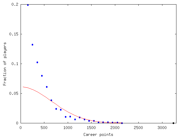
The black point over on the far-right is Gretzky. The fit parameters were µ = 0, σ = 700. Using these, Gretzky gets a z-score of 4.6, making him a 1 in 470 000 player. But that score is a little fuzzy, given the way I derived it.
The second-highest point scorer, Messier, gets a z-score of 3.1, comparable with the non-Bradman greats in other sports.
Now onto points per game. Here Gretzky is still the all-time leader, at 1.91 ppg, but he's only just ahead of Lemieux (1.85). Lemieux only played 1022 games to Gretzky's 1695. For the following graph, I deleted players with less than 10 games.
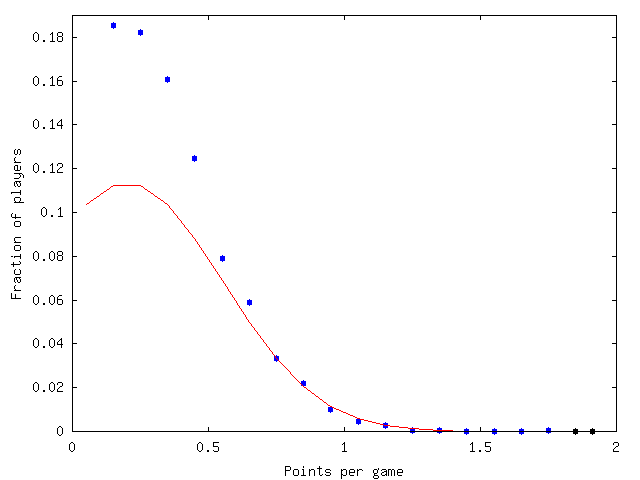
Once again it's been eyeball-fitted, this time with µ = 0.2 and σ = 0.35. This gives Gretzky a z-score of 4.9, Lemieux 4.7, and Gordie Howe 3.6.
Once again, the numbers are fuzzy, but strongly suggestive that Gretzky and Lemieux are up there with Bradman.
This is all well and good, but Mark, at least, would still say that Bobby Orr was better. I don't really know how to measure defencemen in terms of how well they defend, but I can see how many points they scored, and here Orr does fantastically in points per game. He averaged 1.38 ppg, easily the highest for any defenceman (second, and the only other defenceman above 1, is Paul Coffey at 1.08). Here's the ppg graph for the 1420 defencemen with at least 10 NHL games:
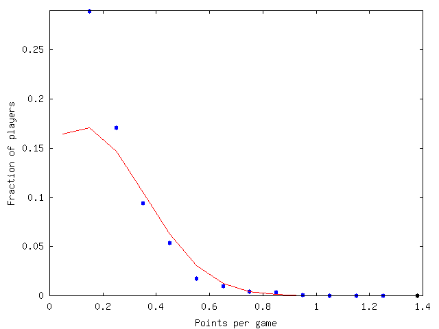
The fit parameters are µ = 0.12 and σ = 0.23. Again the numbers are fuzzy — how much of the tail do you fit? The z-score for Orr will be huge regardless. Here it is a whopping 5.5, though with a less generous fit for him it can be closer to 4.6.
There's certainly more room for analysis, particularly in terms of adjusting for eras. Some of Gretzky's early years were very high-scoring in general, for instance.
Whatever the case, I think these numbers are suggestive that Gretzky and Orr were about as great in what they did as Bradman was.
The technique used to compare players across sports is to find a suitable quantity to measure for each player, so that the resulting distribution for all players becomes a bell curve, at least in the high tail. From this, you can compute each player's z-score (z = (x-µ)/σ, where µ is the mean, and σ is the standard deviation), which is directly comparable across different sports.
Davis' analysis of cricketers gives Bradman a z-score of 5.0 when considering batsmen only, and 4.4 when combining batting, bowling, and fielding. Keep in mind the batsmen-only score here, because that will be a fairer comparison to the ice hockey players. It's worth pointing out, for those unfamiliar with statistics, that a z-score of 5 is truly phenomenal — only one player in almost 3.5 million should be that good compared to all other players of the sport. That's 3.5 million Test cricketers, in this case, not 3.5 million members of the general public. There have only been about 2500 Test cricketers, so for Bradman to have existed makes us very lucky.
Davis' analysis of other sports was not as detailed as for cricket, but the results are reasonably persuasive. Pele is the closest to Bradman, with a z-score of 3.7 for goals per international game. Ty Cobb's baseball batting average turns into a z-score of 3.6. Though these numbers might not look so far away from Bradman's 4.4 or 5, you have to remember that larger z-scores become much, much rarer — Pele's 3.7 makes him a 1 in 14000 player.
Unfortunately, Davis neglected ice hockey, even as a major international sport. If cricket is to be counted as an international sport, then so should ice hockey. Most international cricket is sustained by relatively small population bases. Ice hockey's international reach is similar to cricket's. Wikipedia tells me that "most" of the World Championship medals have gone to Canada, the Czech Republic, Finland, Russia, Slovakia, Sweden, and the United States. That's seven countries, a similar number to cricket.
I am particularly interested in hockey here because it is the only major sport I know of to have a player who dominated statistically in a similar way to Bradman. Wayne Gretzky scored 3239 points (that is, goals and assists) in the NHL (including both regular season and play-offs). The next highest point scorers in NHL history are Mark Messier with 2182 and Gordie Howe with 2010. So I decided to do a similar analysis to Davis' for hockey. Bear in mind that this is a rough job done in a few hours and suitable for a blog post, rather than something a bit more careful suitable for ink and paper.
(A disclaimer: While I like watching hockey, I don't have a deep knowledge of the game. Feel free to correct anything I get wrong.)
Using career points, rather than points per game, is common for two main reasons. Firstly, the number of games played by the best players has stayed relatively constant in the last 60 years (certainly compared to cricket!), so comparisons between eras are meaningful. Gordie Howe, who played in the NHL from 1946 to 1971, has the record for the most NHL games with 1767. Second is Messier (1756), who retired in 2004.
Secondly, in a rough sport where players can play over 70 games a season, longevity is a key ingredient in greatness. Nevertheless, it wasn't Mario Lemieux's fault that he got cancer and had various other injuries, so I have considered points per game later as well.
So, onto the analysis. I downloaded the data on NHL players from The Internet Hockey Database. I deleted four players whose numbers didn't tally, and then used only the players classified as forwards by the Hockey Database. This left 3526 players.
I then binned the career points, and eyeball-fitted a normal distribution to the high tail. I wasn't entirely sure what the best approach was here — I had two free parameters to work with (mean and standard deviation), and so I didn't know the best way to do a least squares in this situation. I'm not a statistician by training. Anyway, the fit at the high end is reasonable — it looks comparable to the fits in The Best of the Best — so we can at least get suggestive results. Here's the graph:
The black point over on the far-right is Gretzky. The fit parameters were µ = 0, σ = 700. Using these, Gretzky gets a z-score of 4.6, making him a 1 in 470 000 player. But that score is a little fuzzy, given the way I derived it.
The second-highest point scorer, Messier, gets a z-score of 3.1, comparable with the non-Bradman greats in other sports.
Now onto points per game. Here Gretzky is still the all-time leader, at 1.91 ppg, but he's only just ahead of Lemieux (1.85). Lemieux only played 1022 games to Gretzky's 1695. For the following graph, I deleted players with less than 10 games.
Once again it's been eyeball-fitted, this time with µ = 0.2 and σ = 0.35. This gives Gretzky a z-score of 4.9, Lemieux 4.7, and Gordie Howe 3.6.
Once again, the numbers are fuzzy, but strongly suggestive that Gretzky and Lemieux are up there with Bradman.
This is all well and good, but Mark, at least, would still say that Bobby Orr was better. I don't really know how to measure defencemen in terms of how well they defend, but I can see how many points they scored, and here Orr does fantastically in points per game. He averaged 1.38 ppg, easily the highest for any defenceman (second, and the only other defenceman above 1, is Paul Coffey at 1.08). Here's the ppg graph for the 1420 defencemen with at least 10 NHL games:
The fit parameters are µ = 0.12 and σ = 0.23. Again the numbers are fuzzy — how much of the tail do you fit? The z-score for Orr will be huge regardless. Here it is a whopping 5.5, though with a less generous fit for him it can be closer to 4.6.
There's certainly more room for analysis, particularly in terms of adjusting for eras. Some of Gretzky's early years were very high-scoring in general, for instance.
Whatever the case, I think these numbers are suggestive that Gretzky and Orr were about as great in what they did as Bradman was.
Thursday, January 03, 2008
It's harder to make 3 than 4.
Dubaiwalla has requested a post on probabilities of getting out for certain scores. Here it is.
The overall distribution of scores (ignoring not outs) is shown below.
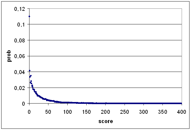
In all, there had been 7160 ducks (almost 11% of all dismissals) and 2710 scores of 1 (just over 4%) up until Christmas 2007.
The overall trend is decreasing, but there are a couple of quirks which are worth looking at. Firstly, there's the irregularities at low scores. In table form:
The frequencies decrease from 0 to 3, but there's a jump at 4 (and a smaller one at 8). We can guess that the jump at 4 is because it is quite common to hit (or edge!) a boundary early in your innings, but less likely that you're good enough to nudge a single and a 2. Interestingly, if you consider only batsmen who average at least 40, the ratio of scores of 4 to scores of 3 is almost identical. The curve is much flatter though — of these batsmen, scores of 4, 5, 6, 7, 8, and 9 are more likely than scores of 3.
It's a similar story for the mini-spike at 8. In innings for which I have boundary data, there is an average of 0,56 fours in innings when the batsman's out for 6; 0,59 when out for 7; and 0,85 when out for 8.
There are other spikes at seemingly random places (e.g., 42 is about 10% more dangerous to be on than either 41 or 43; 54 is almost 20% more dangerous than 53 or 55), presumably statistical noise. The spikes at 50 and 100 are less likely to be noise.
Charles Davis has already looked at the "nervous nineties" in his book. I should get hold of this book next week (let's hope it didn't get lost in the mail!), so I'm not yet sure exactly what he did.
What I've done is plotted a graph of the probability that you'll be dismissed in the next ten runs, given your current score.
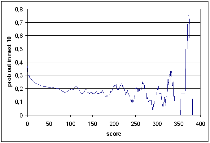
You can see a local minimum at around 90 — batsmen really do go through the nervous nineties, but because they're concentrating harder, they don't get out as often. Then, once past 100, batsmen often lose concentration and get out — the following local maximum is at 114 (agreeing with the bit of Davis's results that I have come across).
There are similar effects near 190 and 240. It is particularly pronounced on the graph at 290, but we're dealing with very little data here — there have been two dismissals in the 290's (Richards 291, Crowe 299), and four between 300 and 309 (Rowe 302, Bradman 304, Cowper 307, Sehwag 309).
There's also a minimum near 127, which is a bit weird and probably noise. There have been 23 dismissals for 136, but 37 for 137 and 31 for 138.
The overall distribution of scores (ignoring not outs) is shown below.
In all, there had been 7160 ducks (almost 11% of all dismissals) and 2710 scores of 1 (just over 4%) up until Christmas 2007.
The overall trend is decreasing, but there are a couple of quirks which are worth looking at. Firstly, there's the irregularities at low scores. In table form:
0   7160
1   2710
2   2183
3   1707
4   2281
5   1846
6   1641
7   1447
8   1497
9   1332
10  1200
The frequencies decrease from 0 to 3, but there's a jump at 4 (and a smaller one at 8). We can guess that the jump at 4 is because it is quite common to hit (or edge!) a boundary early in your innings, but less likely that you're good enough to nudge a single and a 2. Interestingly, if you consider only batsmen who average at least 40, the ratio of scores of 4 to scores of 3 is almost identical. The curve is much flatter though — of these batsmen, scores of 4, 5, 6, 7, 8, and 9 are more likely than scores of 3.
It's a similar story for the mini-spike at 8. In innings for which I have boundary data, there is an average of 0,56 fours in innings when the batsman's out for 6; 0,59 when out for 7; and 0,85 when out for 8.
There are other spikes at seemingly random places (e.g., 42 is about 10% more dangerous to be on than either 41 or 43; 54 is almost 20% more dangerous than 53 or 55), presumably statistical noise. The spikes at 50 and 100 are less likely to be noise.
Charles Davis has already looked at the "nervous nineties" in his book. I should get hold of this book next week (let's hope it didn't get lost in the mail!), so I'm not yet sure exactly what he did.
What I've done is plotted a graph of the probability that you'll be dismissed in the next ten runs, given your current score.
You can see a local minimum at around 90 — batsmen really do go through the nervous nineties, but because they're concentrating harder, they don't get out as often. Then, once past 100, batsmen often lose concentration and get out — the following local maximum is at 114 (agreeing with the bit of Davis's results that I have come across).
There are similar effects near 190 and 240. It is particularly pronounced on the graph at 290, but we're dealing with very little data here — there have been two dismissals in the 290's (Richards 291, Crowe 299), and four between 300 and 309 (Rowe 302, Bradman 304, Cowper 307, Sehwag 309).
There's also a minimum near 127, which is a bit weird and probably noise. There have been 23 dismissals for 136, but 37 for 137 and 31 for 138.
![]()
Subscribe to Posts [Atom]